5 - 下周的光追Part2
开始学习大名鼎鼎的光追三部曲系列中的:Ray Tracing: The Next Week!希望我能坚持下去吧。
纹理映射
在图形学中,纹理映射就是将一种材质效果应用到场景中物体的过程。纹理就是材质效果,映射就是用数学方法将材质从纹理空间映射到物体空间。
最常用的纹理映射就是将图片“贴”在物体表面上。但我们反着来:先获取物体上的点,然后去纹理贴图上查找颜色。
抽象纹理类
我们将制作一些纹理颜色,然后创建一个纯色纹理。为了实现在纹理上查找,需要纹理坐标系。这个坐标系的定义将随进度更改。目前是2D坐标系,每一对将映射一个颜色常量。纹理类的第一个方法是Color value(),它根据给定的坐标输出对应纹理颜色。
因此可以先抽象纹理类如下:
class Texture
{
public:
    virtual ~Texture() = default;

    virtual Color value(double u, double v, const Point3& p) const = 0;
};
纯色纹理
接下来编写纯色纹理类:
class SolidColor : public Texture
{
public:
    SolidColor(const Color& albedo) : albedo(albedo) {}
    SolidColor(double r, double g, double b) : SolidColor(Color(r, g, b)) {}

    Color value(double u, double v, const Point3& p) const override
    {
        return albedo;
    }

private:
    Color albedo;
};
别忘了在HitRecord上补充着色点的(u, v)坐标:
class HitRecord
{
public:
    Point3 position;
    Vec3 normal;
    shared_ptr<Material> material;
    double t;
    double u, v;
    bool front_face;

    ...
};
空间纹理:棋盘格纹理
空间纹理(Solid/Spatial Texture)只依赖于3D空间上每个点的位置,而不是根据物体的形状贴合。因此物体在改变位置时可能“穿过”这种材质,需要自己手动修复二者关系。
为了探索空间纹理,我们将会实现一个棋盘格纹理类CheckerTexture,空间纹理将不会依赖于物体的u, v坐标,而是依赖于着色点位置p。首先,我们要计算位置3个分量的向下取整结果。然后根据分量和的奇偶决定该点的材质。最后给纹理添加一个缩放标量,允许我们控制棋盘格纹理的大小:
class CheckerTexture : public Texture
{
public:
    CheckerTexture(double scale, shared_ptr<Texture> even, shared_ptr<Texture> odd)
        : inv_scale(1.0 / scale), even(even), odd(odd) {}
    CheckerTexture(double scale, const Color& c1, const Color& c2)
        :CheckerTexture(scale, make_shared<SolidColor>(c1), make_shared<SolidColor>(c2)) {}

    Color value(double u, double v, const Point3& p) const override
    {
        int x_i = static_cast<int>(std::floor(inv_scale * p.x()));
        int y_i = static_cast<int>(std::floor(inv_scale * p.y()));
        int z_i = static_cast<int>(std::floor(inv_scale * p.z()));

        bool isEven = (x_i + y_i + z_i) % 2 == 0;
        return isEven ? even->value(u, v, p) : odd->value(u, v, p);
    }

private:
    double inv_scale;
    shared_ptr<Texture> even;
    shared_ptr<Texture> odd;
};
这种根据奇偶选择不同纹理的思想被称为程序化纹理思想(Procedural Texture)。接下来我们拓展Lambertian材质,让它支持程序化纹理:
class Lambertian : public Material
{
public:
    Lambertian(const Color& albedo) : tex(make_shared<SolidColor>(albedo)) {}
    Lambertian(shared_ptr<Texture> tex) : tex(tex) {}

    bool scatter(const Ray& r_in, const HitRecord& rec, Color& attenuation, Ray& scattered) const override
    {
        // Lambert反射模型 (内外表面单位球均考虑)
        Vec3 scatter_direction = rec.normal + random_unit_vector();
        // 只考虑外表面单位球: Vec3 direction = rec.normal + random_on_hemisphere(rec.normal);

        // 处理边界问题
        if (scatter_direction.near_zero())
        {
            scatter_direction = rec.normal;
        }

        scattered = Ray(rec.position, scatter_direction, r_in.time());
        attenuation = tex->value(rec.u, rec.v, rec.position);
        return true;
    }

private:
    shared_ptr<Texture> tex;
};
然后修改Main.cpp看看效果:
void book1Scene(HittableList& world, Camera& cam)
{
    auto checker_tex = make_shared<CheckerTexture>(0.32, Color(0.2, 0.3, 0.1), Color(0.9, 0.9, 0.9));
    world.add(make_shared<Sphere>(Point3(0, -1000, 0), 1000, make_shared<Lambertian>(checker_tex)));
    ...
}
结果如下:
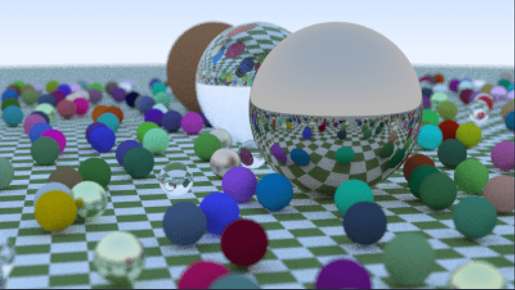
使用棋盘格纹理渲染
接下来添加一个两个球相切的场景,使用棋盘格纹理:
void checkedSpheresScene(HittableList& world, Camera& cam)
{
    auto checker_tex = make_shared<CheckerTexture>(0.32, Color(0.2, 0.3, 0.1), Color(0.9, 0.9, 0.9));
    world.add(make_shared<Sphere>(Point3(0, -10, 0), 10, make_shared<Lambertian>(checker_tex)));
    world.add(make_shared<Sphere>(Point3(0, 10, 0), 10, make_shared<Lambertian>(checker_tex)));

    cam.aspectRadio = 16.0 / 9.0;
    cam.imgWidth = 400;
    cam.samples_per_pixel = 100;
    cam.max_depth = 50;

    cam.vfov = 20;
    cam.lookFrom = Point3(13, 2, 3);
    cam.lookAt = Point3(0, 0, 0);
    cam.vup = Vec3(0, 1, 0);

    cam.defocus_angle = 0;
}
结果如下:
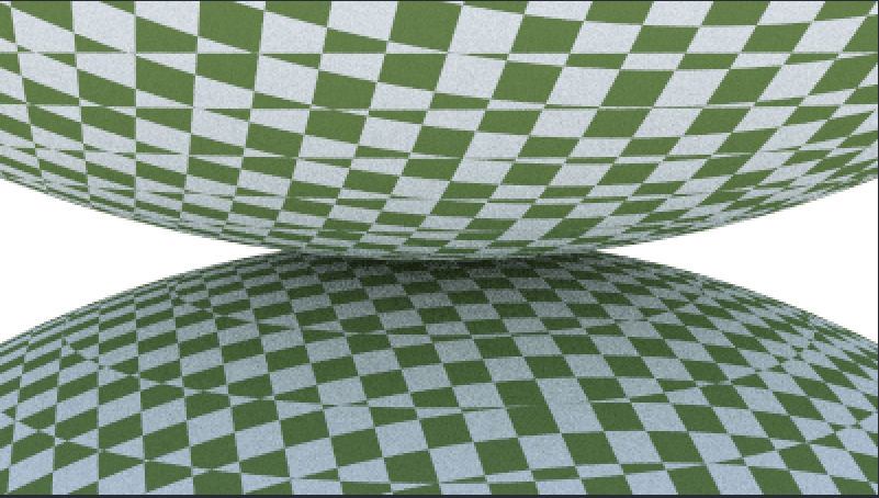
空间纹理的缺点便体现出来,它是基于位置的,而不是物体表面。接下来将介绍改进方法。
球体的纹理坐标系
纯色纹理不使用坐标系;空间纹理使用3D空间中的点;接下来是时候让坐标起作用了。这些坐标特定于一张2D纹理图上。为了得到它,我们需要找到从3D坐标映射到坐标的方法。
对于球体,纹理坐标通常基于某种经纬度形式,即球面坐标系。所以我们计算球面坐标系的,其中是极角,跨度从+y到-y;是方位角,跨度从-x, +z到$+x, -z。
我们需要将映射到属于的坐标中,其中在纹理的左下角。因此从到的标准化公式为:
然后根据定义将位于单位球表面的转换到直角坐标系中:
然后就能用直角坐标逆向求出了,首先看看如何求,只需联立即可:
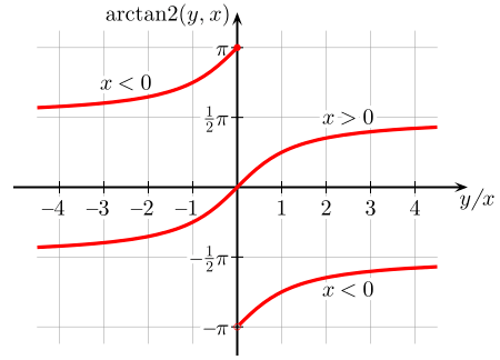
如图,std::atan2()返回值范围是,但它是从到,然后从到,不是“连续”的。我们想让从到,而不是从到,然后从到。可以用
将返回值范围映射到连续的,因此有
的计算就更简单了:
因此可以在Sphere类中添加工具函数get_sphere_uv(),将3D坐标转换为UV坐标:
/**
 * 将直角坐标转换为UV坐标
 * @param p 单位球面上1点,用直角坐标表示
 * @param u 返回方位角\phi到[0, 1]的映射
 * @param v 返回极角\theta到[0, 1]的映射
 */
static void get_sphere_uv(const Point3& p, double& u, double& v)
{
    double theta = std::acos(-p.y());
    double phi = std::atan2(-p.z(), p.x()) + pi;

    u = phi / (2 * pi);
    v = theta / pi;
}
然后就能更新球体类hit()中的u和v了:
// 记录相交信息
rec.t = root;
rec.position = r.at(rec.t);
Vec3 outward_normal = (rec.position - center) / radius;    // 利用定义简化法线计算
rec.set_face_normal(r, outward_normal);
get_sphere_uv(outward_normal, rec.u, rec.v);
rec.material = material;
这个可以作为程序化纹理或2D纹理图片的索引。
获取纹理图片信息
可以通过stb_image库加载图片信息,这里用封装好的RRWImage类管理2D纹理图片,它有一个叫做pixel_data(int x, int y)的帮手函数,用于获取每像素的8位RGB信息:
#pragma once

// 屏蔽MSVC编译器警告
#ifdef _MSC_VER
#pragma warning (push, 0)
#endif // _MSC_VER

#define STB_IMAGE_IMPLEMENTATION
#define STBI_FAILURE_USERMSG
#include "stbi/stb_image.h"

#include <cstdlib>
#include <iostream>

class RTWImage
{
public:
    RTWImage() {}
    RTWImage(const char* img_filepath)
    {
        auto filepath = std::string(img_filepath);
        if (load(filepath))    return;

        std::cerr << "ERROR: 加载图片文件 " << filepath << " 失败!\n";
    }

    ~RTWImage()
    {
        delete[] bdata;
        STBI_FREE(fdata);
    }

    bool load(const std::string& filename)
    {
        auto n = bytes_per_pixel;
        fdata = stbi_loadf(filename.c_str(), &image_width, &image_height, &n, bytes_per_pixel);
        if (fdata == nullptr)
        {
            return false;
        }

        bytes_per_scanline = image_width * bytes_per_pixel;
        convert_to_bytes();
        return true;
    }

    int width() const { return (fdata == nullptr) ? 0 : image_width; }
    int height() const { return (fdata == nullptr) ? 0 : image_height; }

    const unsigned char* pixel_data(int x, int y) const
    {
        static unsigned char magenta = {255, 0, 255};
        if (bdata == nullptr)
        {
            return magenta;
        }

        x = clamp(x, 0, image_width);
        y = clamp(y, 0, image_height);
        return bdata + y * bytes_per_scanline + x * bytes_per_pixel;
    }

private:
    const int bytes_per_pixel = 3;
    float* fdata = nullptr;            // 线性浮点数像素数据
    unsigned char* bdata = nullptr;    // 线性8位像素数据
    int image_width = 0;
    int image_height = 0;
    int bytes_per_scanline = 0;

    // 返回将x限定至[low, high)的结果
    static int clamp(int x, int low, int high)
    {
        if (x < low)    return low;
        if (x < high)    return x;
        return high - 1;
    }

    // 将位于[0, 1]的颜色转换为[0, 255]
    static unsigned char float_to_byte(float value)
    {
        if (value <= 0.0)    return 0;
        if (1.0 <= value)    return 255;
        return static_cast<unsigned char>(256.0 * value);
    }

    // 将线性浮点像素数据转换为8位的
    void convert_to_bytes()
    {
        int total_bytes = image_width * image_height * bytes_per_pixel;
        bdata = new unsigned char[total_bytes];

        auto* bptr = bdata;
        auto* fptr = fdata;
        for (auto i = 0; i < total_bytes; ++i, ++fptr, ++bptr)
        {
            *bptr = float_to_byte(*fptr);
        }
    }
};

// 取消屏蔽MSVC警告
#if _MSC_VER
#pragma warning(pop)
#endif // _MSC_VER
然后新写一个ImageTexture类管理这种材质:
#include "rtw_image.hpp"
#include "texture.hpp"

class ImageTexture : public Texture
{
public:
    ImageTexture(const char* filepath) : image(filepath) {}

    Color value(double u, double v, const Point3& p) const override
    {
        // 没有材质就返回青色
        if (image.height() <= 0)    return Color(0, 1, 1);

        // 将u,v限定至正确的范围, 其中v需要反转
        u = Interval(0, 1).clamp(u);
        v = 1.0 - Interval(0, 1).clamp(v);

        int i = static_cast<int>(u * image.width());
        int j = static_cast<int>(v * image.height());
        auto pixel = image.pixel_data(i, j);

        double color_scale = 1.0 / 255.0;
        return Color(color_scale * pixel[0], color_scale * pixel[1], color_scale * pixel[2]);
    }

private:
    RTWImage image;
};
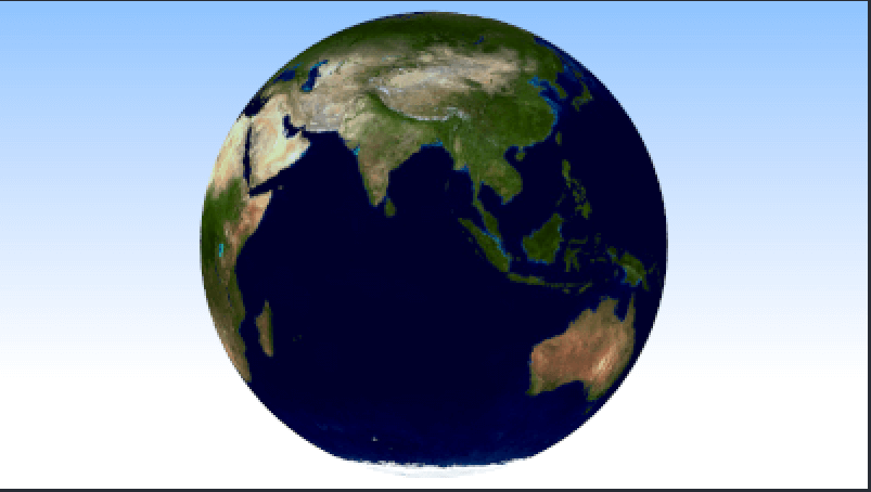
渲染图片纹理
接下来渲染带有地球图片纹理的球,场景如下:
void earth(HittableList& world, Camera& cam)
{
    auto earth_tex = make_shared<ImageTexture>("resources/images/earthmap.jpg");
    auto earth_surface = make_shared<Lambertian>(earth_tex);
    auto globe = make_shared<Sphere>(Point3(0, 0, 0), 2, earth_surface);
    world.add(globe);

    cam.aspectRadio = 16.0 / 9.0;
    cam.imgWidth = 400;
    cam.samples_per_pixel = 100;
    cam.max_depth = 50;

    cam.vfov = 20;
    cam.lookFrom = Point3(0, 0, -12);
    cam.lookAt = Point3(0, 0, 0);
    cam.vup = Vec3(0, 1, 0);

    cam.defocus_angle = 0;
}
结果如下:
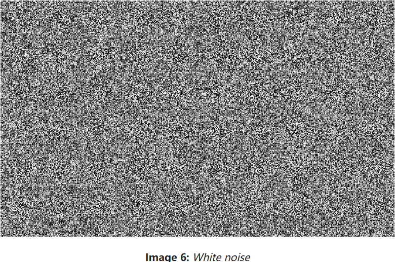
柏林噪声
为了得到一些看起来酷的材质,大多数人选择使用柏林噪声。它不像白噪声一样返回这样的东西:
柏林噪声返回的是类似于模糊白噪声的东西:
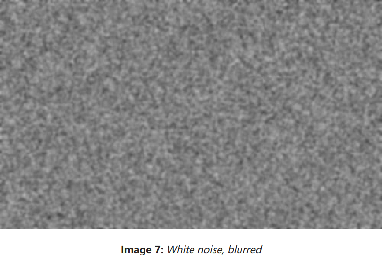
柏林噪声的关键就是:
- 可重复:将一个3D点作为输入,总是返回相同的随机数,附近的点返回类似数字。
- 简单快速:通常作为hack来完成。
使用随机数字块
可以使用一组随机颜色数组,然后重复堆叠它们:
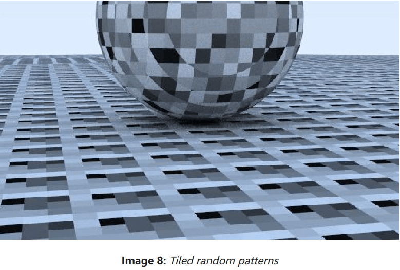
接下来通过一些哈希操作来打乱这种堆叠,创建Perlin类如下:
class Perlin
{
public:
    Perlin()
    {
        for (int i = 0; i < point_count; ++i)
        {
            rand_float[i] = random_double();
        }

        perlin_generate_perm(perm_x);
        perlin_generate_perm(perm_y);
        perlin_generate_perm(perm_z);
    }

    double noise(const Point3& p) const
    {
        int i = static_cast<int>(4 * p.x()) & 255;
        int j = static_cast<int>(4 * p.y()) & 255;
        int k = static_cast<int>(4 * p.z()) & 255;

        return rand_float[perm_x[i] ^ perm_y[j] ^ perm_z[k]];
    }

private:
    static const int point_count = 256;
    double rand_float[point_count];
    int perm_x[point_count];
    int perm_y[point_count];
    int perm_z[point_count];

    static void perlin_generate_perm(int* p)
    {
        for (int i = 0; i < point_count; ++i)
        {
            p[i] = i;
        }
        permute(p, point_count);
    }

    static void permute(int* p, int n)
    {
        for (int i = n - 1; i > 0; --i)
        {
            int target = random_int(0, i);
            std::swap(p[i], p[target]);
        }
    }
};
然后创建NoiseTexture纹理类:
#include "../util/perlin.hpp"
#include "texture.hpp"

class NoiseTexture : public Texture
{
public:
    NoiseTexture() = default;

    Color value(double u, double v, const Point3& p) const override
    {
        return Color(1, 1, 1) * noise.noise(p);
    }

private:
    Perlin noise;
};
最后创建一个新场景:
void perlinSphere(HittableList& world, Camera& cam)
{
    auto perlin_tex = make_shared<NoiseTexture>();
    world.add(make_shared<Sphere>(Point3(0, -1000, 0), 1000, make_shared<Lambertian>(perlin_tex)));
    world.add(make_shared<Sphere>(Point3(0, 2, 0), 2, make_shared<Lambertian>(perlin_tex)));

    cam.aspectRadio = 16.0 / 9.0;
    cam.imgWidth = 400;
    cam.samples_per_pixel = 100;
    cam.max_depth = 50;

    cam.vfov = 20;
    cam.lookFrom = Point3(13, 2, 3);
    cam.lookAt = Point3(0, 0, 0);
    cam.vup = Vec3(0, 1, 0);

    cam.defocus_angle = 0;
}
可能的结果如下:

三线性插值
为了让结果更加平滑,可以使用线性插值。修改Perlin类,让它支持三线性插值:
class Perlin
{
public:
    ...
    double noise(const Point3& p) const
    {
        double u = p.x() - std::floor(p.x());
        double v = p.y() - std::floor(p.y());
        double w = p.z() - std::floor(p.z());

        int i = static_cast<int>(std::floor(p.x()));
        int j = static_cast<int>(std::floor(p.y()));
        int k = static_cast<int>(std::floor(p.z()));
        double c[2][2][2];

        for (int di = 0; di < 2; ++di)
        {
            for (int dj = 0; dj < 2; ++dj)
            {
                for (int dk = 0; dk < 2; ++dk)
                {
                    c[di][dj][dk] = rand_float[perm_x[(i + di) & 255] ^ perm_y[(j + dj) & 255] ^ perm_z[(k + dk) & 255]];
                }
            }
        }

        return trilinear_interp(c, u, v, w);
    }

private:
    ...
    static double trilinear_interp(double c[2][2][2], double u, double v, double w)
    {
        double accum = 0;
        for (int i = 0; i < 2; ++i)
        {
            for (int j = 0; j < 2; ++j)
            {
                for (int k = 0; k < 2; ++k)
                {
                    accum += (i * u + (1 - i) * (1 - u))
                        * (j * v + (1 - j) * (1 - v))
                        * (k * w + (1 - k) * (1 - w))
                        * c[i][j][k];
                }
            }
        }
        return accum;
    }
};
使用三线性插值的结果如下:
Hermitian平滑
上面结果平滑点了,但仍有明显的网格状特征。有些人称其为马赫带效应,一种著名的线性插值时出现的瑕疵。解决它的一种标准技巧是使用三次Hermite曲线来舍入插值的结果。
只需修改Perlin类的noise()即可:
double noise(const Point3& p) const
{
    double u = p.x() - std::floor(p.x());
    double v = p.y() - std::floor(p.y());
    double w = p.z() - std::floor(p.z());
    u = u * u * (3 - 2 * u);
    v = v * v * (3 - 2 * v);
    w = w * w * (3 - 2 * w);
    ...
}
这使得结果更加平滑:
调整频率
噪声纹理出现的频率有些低了,可以通过使用scale增加其频率,修改NoiseTexture类如下:
class NoiseTexture : public Texture
{
public:
    NoiseTexture(double scale) : scale(scale) {}

    Color value(double u, double v, const Point3& p) const override
    {
        return Color(1, 1, 1) * noise.noise(scale * p);
    }

private:
    Perlin noise;
    double scale;
};
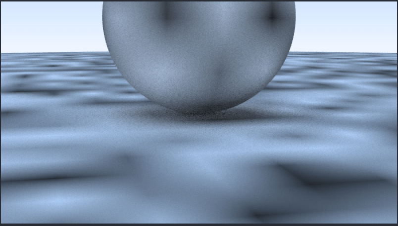
scale为4时的结果如下:
在格点上使用随机向量
结果看上去仍然有些块状,可能是因为最值总是落在整数x/y/z上。柏林噪声聪明的做法是,将随机单位向量(不只是浮点数)放到格点上,并且使用点乘去将最值移出格点。所以我们首先需要将随机浮点数改为随机向量。
修改Perlin类如下:
class Perlin
{
public:
    Perlin()
    {
        for (int i = 0; i < point_count; ++i)
        {
            rand_vec[i] = unitVector(Vec3::random(-1, 1));
        }

        perlin_generate_perm(perm_x);
        perlin_generate_perm(perm_y);
        perlin_generate_perm(perm_z);
    }
    ...

private:
    static const int point_count = 256;
    Vec3 rand_vec[point_count];
    ...
};
再修改它的noise()方法如下:
double noise(const Point3& p) const
{
    double u = p.x() - std::floor(p.x());
    double v = p.y() - std::floor(p.y());
    double w = p.z() - std::floor(p.z());

    int i = static_cast<int>(std::floor(p.x()));
    int j = static_cast<int>(std::floor(p.y()));
    int k = static_cast<int>(std::floor(p.z()));
    Vec3 c[2][2][2];

    for (int di = 0; di < 2; ++di)
    {
        for (int dj = 0; dj < 2; ++dj)
        {
            for (int dk = 0; dk < 2; ++dk)
            {
                c[di][dj][dk] = rand_vec[perm_x[(i + di) & 255] ^ perm_y[(j + dj) & 255] ^ perm_z[(k + dk) & 255]];
            }
        }
    }

    return perlin_interp(c, u, v, w);
}
然后完善perlin_interp()方法:
static double perlin_interp(const Vec3 c[2][2][2], double u, double v, double w)
{
    double uu = u * u * (3 - 2 * u);
    double vv = v * v * (3 - 2 * v);
    double ww = w * w * (3 - 2 * w);
    double accum = 0.0;

    for (int i = 0; i < 2; ++i)
    {
        for (int j = 0; j < 2; ++j)
        {
            for (int k = 0; k < 2; ++k)
            {
                Vec3 weight_v(u - i, v - j, w - k);
                accum += (i * uu + (1 - i) * (1 - uu))
                    * (j * vv + (1 - j) * (1 - vv))
                    * (k * ww + (1 - k) * (1 - ww))
                    * dot(c[i][j][k], weight_v);
            }
        }
    }

    return accum;
}
由于perlin_interp()的返回值会返回的值,我们要将其映射到上。修改NoiseTexture如下:
class NoiseTexture : public Texture
{
public:
    NoiseTexture(double scale) : scale(scale) {}

    Color value(double u, double v, const Point3& p) const override
    {
        return Color(1, 1, 1) * 0.5 * (1.0 + noise.noise(scale * p));
    }

private:
    Perlin noise;
    double scale;
};
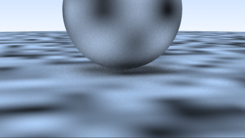
偏移格点极值后的结果如下,更合理了:
引入湍流效果
通常我们会使用具有多种频率的合成噪声,这通常被称为“湍流(Turbulence)”,就是重复调用noise()的总和。在Perlin类中添加turb()方法:
double turb(const Point3& p, int depth) const
{
    double accum = 0.0;
    Point3 tmp_p = p;
    double weight = 1.0;

    for (int i = 0; i < depth; ++i)
    {
        accum += weight * noise(tmp_p);
        weight *= 0.5;
        tmp_p *= 2;
    }

    return std::fabs(accum);
}
然后修改对应纹理类试试:
class NoiseTexture : public Texture
{
public:
    NoiseTexture(double scale) : scale(scale) {}

    Color value(double u, double v, const Point3& p) const override
    {
        return Color(1, 1, 1) * noise.turb(p, 7);
    }

private:
    Perlin noise;
    double scale;
};
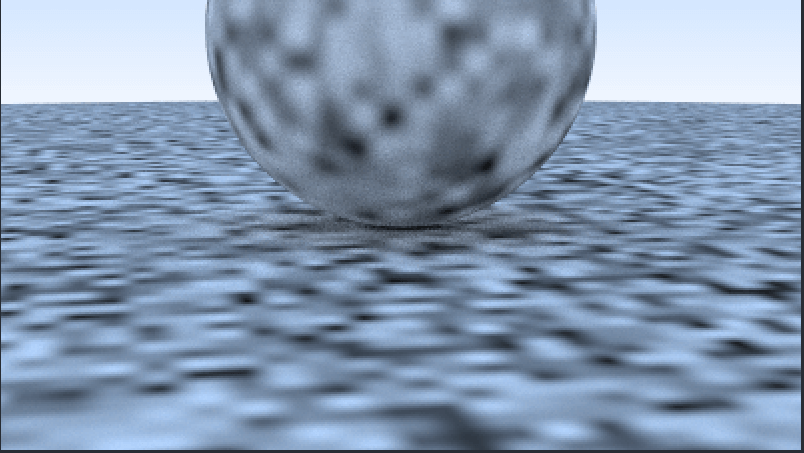
结果如下:
适应相位
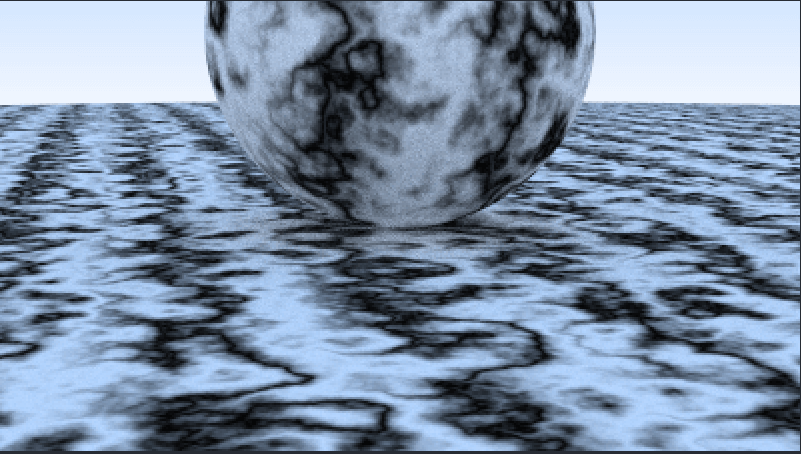
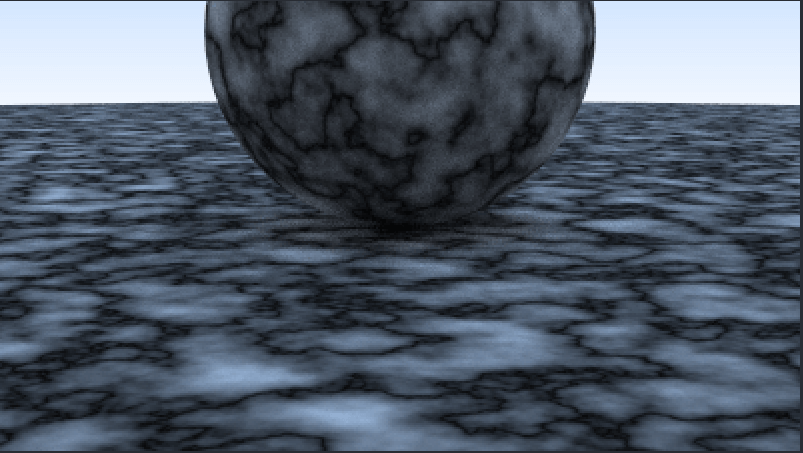
然而,湍流效果不是直接使用的。例如程序化生成空间纹理的“hello world”是大理石似的纹理。基本思想是让颜色随某种正弦函数变化,并且使用湍流效果适应相位。可以这样做:
Color value(double u, double v, const Point3& p) const override
{
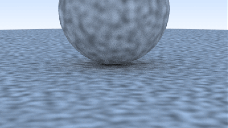
return Color(0.5, 0.5, 0.5) * (1 + std::sin(scale * p.z() + 10 * noise.turb(p, 7)));
}
结果如下: